The numerical data from graphs digitized with Dagra can be loaded into Matlab using our Matlab function, the system clipboard or a text file.
The easiest method is using the LoadDagra.m function because you don’t need to create a separate file or fill up Matlab’s command buffer with the imported data. The options are:
- The
LoadDagra.mfunction for Matlab. This function loads Dagra documents into a structure. - Digitized data can also be copied onto the clipboard (Edit→Copy Data… in Dagra) and pasted into the command line window, or
- exported into a text file (File→Export Data… in Dagra) and imported using Matlab’s dlmread function.
Setup
LoadDagra.m must be on Matlab’s search path before it can be used. The function is installed in the Dagra application directory in the folder Components\Matlab\.
If Dagra was installed in the default location, then the command to include it in the search path is:
|
1 |
>> addpath('c:\Program Files\Blue Leaf Software\Dagra\Components\Matlab'); |
Load the Data
LoadDagra.m takes a single argument, the path to the Dagra document to load. Only the filename is needed if the file is in the current directory. It returns a structure containing fields for each series in the Dagra document:
|
1 2 3 4 5 6 |
>> data = LoadDagra('Bromocresol green.dag') data = Basic: [1x1 struct] Acid: [1x1 struct] Intermediate: [1x1 struct] >> |
Spaces in the series name are replaced by underscore characters to form valid field names.
The Series Structure
Each series structure contains two fields: x and y. Each is a vector containing the exported data. These vectors will always be the same length.
|
1 2 3 4 5 |
>> data.Acid ans = x: [89x1 double] y: [89x1 double] >> |
Note: if you are using an expired trial version of Dagra, the exported data contains random noise. Purchase a Dagra license to recover the original high-precision data.
Plotting the Data
This Matlab code creates a plot showing the graphical source image on the left and data digitized with Dagra on the right:
|
1 2 3 4 5 6 7 8 |
>> figure(1); >> img = imread('Bromocresol green spectrum.png'); >> subplot(1,2,1); >> image(img); >> axis('off'); >> subplot(1,2,2); >> plot(data.Acid.x, data.Acid.y, 'b', data.Basic.x, data.Basic.y, 'r', data.Intermediate.x, data.Intermediate.y, 'g'); >> xlabel('Wavelength [nm]'); ylabel('Absorption'); grid on; |
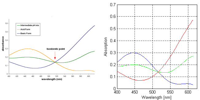
The spectrum of Bromocresol green from Wikipedia (left) and the digitized data plotted in Matlab (right).
Interpolating the Data
Dagra exports sufficient data to accurately reconstruct the curves. So intermediate values can be obtained with linear interpolation using Matlab’s interp1 function.
To estimate the absorbance of the acid form of Bromocresol green at 450, 515 and 570 nm, for example:
|
1 2 3 4 |
>> interp1(data.Acid.x, data.Acid.y, [450 515 550]) ans = 0.29789 0.14131 0.053782 >> |